Using Apache Spark in Fabric

Apache Spark is an open source parallel processing framework for large-scale data processing and analytics. Spark has become popular in “big data” processing scenarios, and is available in multiple platform implementations; including Azure HDInsight, Azure Databricks, Azure Synapse Analytics, and Microsoft Fabric.

This module explores how you can use Spark in Microsoft Fabric to ingest, process, and analyze data in a lakehouse. While the core techniques and code described in this module are common to all Spark implementations, the integrated tools and ability to work with Spark in the same environment as other data services in Microsoft Fabric makes it easier to incorporate Spark-based data processing into your overall data analytics solution.

Prepare to use Apache Spark

Apache Spark is distributed data processing framework that enables large-scale data analytics by coordinating work across multiple processing nodes in a cluster. Put more simply, Spark uses a “divide and conquer” approach to processing large volumes of data quickly by distributing the work across multiple computers. The process of distributing tasks and collating results is handled for you by Spark. You submit a data processing job in the form of some code that initiates a driver program, which uses a cluster management object called the SparkContext to manage the distribution of processing in the Spark cluster. In most cases, these details are abstracted – you just need to write the code required to perform the data operations you need.

Spark can run code written in a wide range of languages, including Java, Scala (a Java-based scripting language), Spark R, Spark SQL, and PySpark (a Spark-specific variant of Python). Most data engineering and analytics workloads are accomplished using a combination of PySpark and Spark SQL.

Spark settings

In Microsoft Fabric, each workspace is assigned a Spark cluster. An administrator can manage settings for the Spark cluster in the Data Engineering/Science section of the workspace settings.

Screenshot of the Spark settings page in Microsoft Fabric.

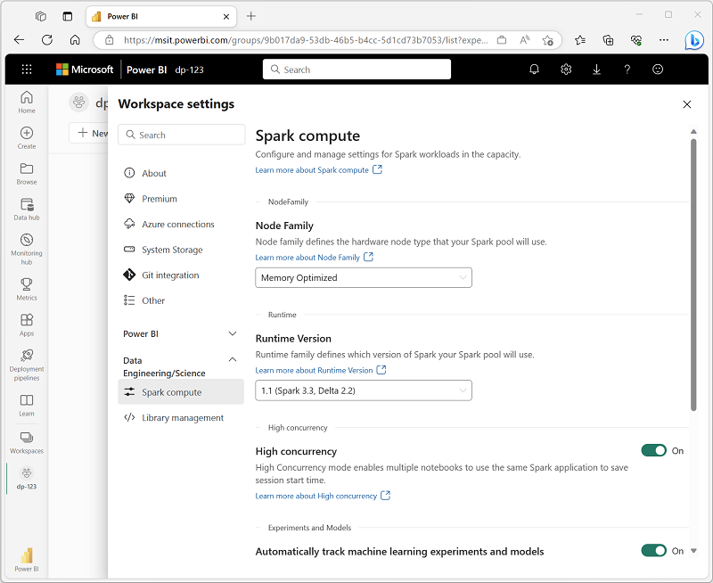
Specific configuration settings include:

  • Node Family: The type of virtual machines used for the Spark cluster nodes. In most cases, memory optimized nodes provide optimal performance.
  • Runtime version: The version of Spark (and dependent subcomponents) to be run on the cluster.
  • Spark Properties: Spark-specific settings that you want to enable or override in your cluster. You can see a list of properties in the Apache Spark documentation.

 Note

In most scenarios, the default settings provide an optimal configuration for Spark in Microsoft Fabric.

Libraries

The Spark open source ecosystem includes a wide selection of code libraries for common (and sometimes very specialized) tasks. Since a great deal of Spark processing is performed using PySpark, the huge range of Python libraries ensures that whatever the task you need to perform, there’s probably a library to help.

By default, Spark clusters in Microsoft Fabric include many of the most commonly used libraries, but if you need to install other libraries, you can do so on the Library management page in the workspace settings.

 Tip

For more information about library management, see Manage Apache Spark libraries in Microsoft Fabric in the Microsoft Fabric documentation.


Run Spark code

Completed100 XP

To edit and run Spark code in Microsoft Fabric, you can use notebooks, or you can define a Spark job.

Notebooks

When you want to use Spark to explore and analyze data interactively, use a notebook. Notebooks enable you to combine text, images, and code written in multiple languages to create an interactive artifact that you can share with others and collaborate.

Screenshot of a notebook in Microsoft Fabric.

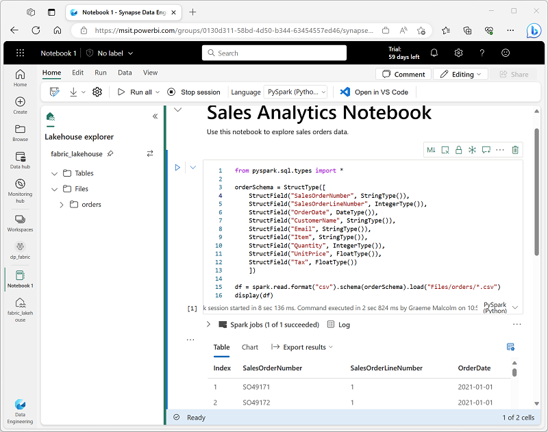
Notebooks consist of one or more cells, each of which can contain markdown-formatted content or executable code. You can run the code interactively in the notebook and see the results immediately.

Spark job definition

If you want to use Spark to ingest and transform data as part of an automated process, you can define a Spark job to run a script on-demand or based on a schedule.

Screenshot of a Spark job definition in Microsoft Fabric.

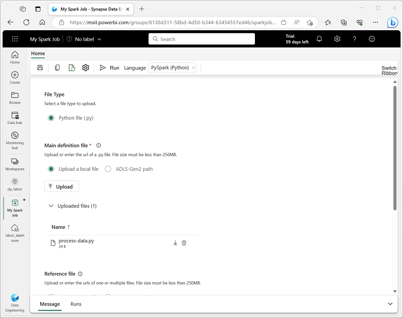
To configure a Spark job, create a Spark Job Definition in your workspace and specify the script it should run. You can also specify a reference file (for example, a Python code file containing definitions of functions that are used in your script) and a reference to a specific lakehouse containing data that the script processes.


Work with data in a Spark dataframe

Completed100 XP

Natively, Spark uses a data structure called a resilient distributed dataset (RDD); but while you can write code that works directly with RDDs, the most commonly used data structure for working with structured data in Spark is the dataframe, which is provided as part of the Spark SQL library. Dataframes in Spark are similar to those in the ubiquitous Pandas Python library, but optimized to work in Spark’s distributed processing environment.

 Note

In addition to the Dataframe API, Spark SQL provides a strongly-typed Dataset API that is supported in Java and Scala. We’ll focus on the Dataframe API in this module.

Loading data into a dataframe

Let’s explore a hypothetical example to see how you can use a dataframe to work with data. Suppose you have the following data in a comma-delimited text file named products.csv in the Files/data folder in your lakehouse:

csv
ProductID,ProductName,Category,ListPrice
771,"Mountain-100 Silver, 38",Mountain Bikes,3399.9900
772,"Mountain-100 Silver, 42",Mountain Bikes,3399.9900
773,"Mountain-100 Silver, 44",Mountain Bikes,3399.9900
...

Inferring a schema

In a Spark notebook, you could use the following PySpark code to load the file data into a dataframe and display the first 10 rows:

Python
%%pyspark
df = spark.read.load('Files/data/products.csv',
    format='csv',
    header=True
)
display(df.limit(10))

The %%pyspark line at the beginning is called a magic, and tells Spark that the language used in this cell is PySpark. You can select the language you want to use as a default in the toolbar of the Notebook interface, and then use a magic to override that choice for a specific cell. For example, here’s the equivalent Scala code for the products data example:

Scala
%%spark
val df = spark.read.format("csv").option("header", "true").load("Files/data/products.csv")
display(df.limit(10))

The magic %%spark is used to specify Scala.

Both of these code samples would produce output like this:

ProductIDProductNameCategoryListPrice
771Mountain-100 Silver, 38Mountain Bikes3399.9900
772Mountain-100 Silver, 42Mountain Bikes3399.9900
773Mountain-100 Silver, 44Mountain Bikes3399.9900

Specifying an explicit schema

In the previous example, the first row of the CSV file contained the column names, and Spark was able to infer the data type of each column from the data it contains. You can also specify an explicit schema for the data, which is useful when the column names aren’t included in the data file, like this CSV example:

csv
771,"Mountain-100 Silver, 38",Mountain Bikes,3399.9900
772,"Mountain-100 Silver, 42",Mountain Bikes,3399.9900
773,"Mountain-100 Silver, 44",Mountain Bikes,3399.9900
...

The following PySpark example shows how to specify a schema for the dataframe to be loaded from a file named product-data.csv in this format:

Python
from pyspark.sql.types import *
from pyspark.sql.functions import *

productSchema = StructType([
    StructField("ProductID", IntegerType()),
    StructField("ProductName", StringType()),
    StructField("Category", StringType()),
    StructField("ListPrice", FloatType())
    ])

df = spark.read.load('Files/data/product-data.csv',
    format='csv',
    schema=productSchema,
    header=False)
display(df.limit(10))

The results would once again be similar to:

ProductIDProductNameCategoryListPrice
771Mountain-100 Silver, 38Mountain Bikes3399.9900
772Mountain-100 Silver, 42Mountain Bikes3399.9900
773Mountain-100 Silver, 44Mountain Bikes3399.9900

 Tip

Specifying an explicit schema also improves performance!

Filtering and grouping dataframes

You can use the methods of the Dataframe class to filter, sort, group, and otherwise manipulate the data it contains. For example, the following code example uses the select method to retrieve the ProductName and ListPrice columns from the df dataframe containing product data in the previous example:

Python
pricelist_df = df.select("ProductID", "ListPrice")

The results from this code example would look something like this:

ProductIDListPrice
7713399.9900
7723399.9900
7733399.9900

In common with most data manipulation methods, select returns a new dataframe object.

 Tip

Selecting a subset of columns from a dataframe is a common operation, which can also be achieved by using the following shorter syntax:

pricelist_df = df["ProductID", "ListPrice"]

You can “chain” methods together to perform a series of manipulations that results in a transformed dataframe. For example, this example code chains the select and where methods to create a new dataframe containing the ProductName and ListPrice columns for products with a category of Mountain Bikes or Road Bikes:

Python
bikes_df = df.select("ProductName", "Category", "ListPrice").where((df["Category"]=="Mountain Bikes") | (df["Category"]=="Road Bikes"))
display(bikes_df)

The results from this code example would look something like this:

ProductNameCategoryListPrice
Mountain-100 Silver, 38Mountain Bikes3399.9900
Road-750 Black, 52Road Bikes539.9900

To group and aggregate data, you can use the groupBy method and aggregate functions. For example, the following PySpark code counts the number of products for each category:

Python
counts_df = df.select("ProductID", "Category").groupBy("Category").count()
display(counts_df)

The results from this code example would look something like this:

Categorycount
Headsets3
Wheels14
Mountain Bikes32

Saving a dataframe

You’ll often want to use Spark to transform raw data and save the results for further analysis or downstream processing. The following code example saves the dataFrame into a parquet file in the data lake, replacing any existing file of the same name.

Python
bikes_df.write.mode("overwrite").parquet('Files/product_data/bikes.parquet')

 Note

The Parquet format is typically preferred for data files that you will use for further analysis or ingestion into an analytical store. Parquet is a very efficient format that is supported by most large scale data analytics systems. In fact, sometimes your data transformation requirement may simply be to convert data from another format (such as CSV) to Parquet!

Partitioning the output file

Partitioning is an optimization technique that enables Spark to maximize performance across the worker nodes. More performance gains can be achieved when filtering data in queries by eliminating unnecessary disk IO.

To save a dataframe as a partitioned set of files, use the partitionBy method when writing the data. The following example saves the bikes_df dataframe (which contains the product data for the mountain bikes and road bikes categories), and partitions the data by category:

Python
bikes_df.write.partitionBy("Category").mode("overwrite").parquet("Files/bike_data")

The folder names generated when partitioning a dataframe include the partitioning column name and value in a column=value format, so the code example creates a folder named bike_data that contains the following subfolders:

  • Category=Mountain Bikes
  • Category=Road Bikes

Each subfolder contains one or more parquet files with the product data for the appropriate category.

 Note

You can partition the data by multiple columns, which results in a hierarchy of folders for each partitioning key. For example, you might partition sales order data by year and month, so that the folder hierarchy includes a folder for each year value, which in turn contains a subfolder for each month value.

Load partitioned data

When reading partitioned data into a dataframe, you can load data from any folder within the hierarchy by specifying explicit values or wildcards for the partitioned fields. The following example loads data for products in the Road Bikes category:

Python
road_bikes_df = spark.read.parquet('Files/bike_data/Category=Road Bikes')
display(road_bikes_df.limit(5))

 Note

The partitioning columns specified in the file path are omitted in the resulting dataframe. The results produced by the example query would not include a Category column – the category for all rows would be Road Bikes.

Work with data using Spark SQL

Completed100 XP

The Dataframe API is part of a Spark library named Spark SQL, which enables data analysts to use SQL expressions to query and manipulate data.

Creating database objects in the Spark catalog

The Spark catalog is a metastore for relational data objects such as views and tables. The Spark runtime can use the catalog to seamlessly integrate code written in any Spark-supported language with SQL expressions that may be more natural to some data analysts or developers.

One of the simplest ways to make data in a dataframe available for querying in the Spark catalog is to create a temporary view, as shown in the following code example:

Python
df.createOrReplaceTempView("products_view")

view is temporary, meaning that it’s automatically deleted at the end of the current session. You can also create tables that are persisted in the catalog to define a database that can be queried using Spark SQL.

Tables are metadata structures that store their underlying data in the storage location associated with the catalog. In Microsoft Fabric, data for managed tables is stored in the Tables storage location shown in your data lake, and any tables created using Spark are listed there.

You can create an empty table by using the spark.catalog.createTable method, or you can save a dataframe as a table by using its saveAsTable method. Deleting a managed table also deletes its underlying data.

For example, the following code saves a dataframe as a new table named products:

Python
df.write.format("delta").saveAsTable("products")

 Note

The Spark catalog supports tables based on files in various formats. The preferred format in Microsoft Fabric is delta, which is the format for a relational data technology on Spark named Delta Lake. Delta tables support features commonly found in relational database systems, including transactions, versioning, and support for streaming data.

Additionally, you can create external tables by using the spark.catalog.createExternalTable method. External tables define metadata in the catalog but get their underlying data from an external storage location; typically a folder in the Files storage area of a lakehouse. Deleting an external table doesn’t delete the underlying data.

 Tip

You can apply the same partitioning technique to delta lake tables as discussed for parquet files in the previous unit. Partitioning tables can result in better performance when querying them.

Using the Spark SQL API to query data

You can use the Spark SQL API in code written in any language to query data in the catalog. For example, the following PySpark code uses a SQL query to return data from the products table as a dataframe.

Python
bikes_df = spark.sql("SELECT ProductID, ProductName, ListPrice \
                      FROM products \
                      WHERE Category IN ('Mountain Bikes', 'Road Bikes')")
display(bikes_df)

The results from the code example would look similar to the following table:

ProductNameListPrice
Mountain-100 Silver, 383399.9900
Road-750 Black, 52539.9900

Using SQL code

The previous example demonstrated how to use the Spark SQL API to embed SQL expressions in Spark code. In a notebook, you can also use the %%sql magic to run SQL code that queries objects in the catalog, like this:

SQL
%%sql

SELECT Category, COUNT(ProductID) AS ProductCount
FROM products
GROUP BY Category
ORDER BY Category

The SQL code example returns a resultset that is automatically displayed in the notebook as a table:

CategoryProductCount
Bib-Shorts3
Bike Racks1
Bike Stands1
 

Visualize data in a Spark notebook

Completed100 XP

One of the most intuitive ways to analyze the results of data queries is to visualize them as charts. Notebooks in Microsoft Fabric provide some basic charting capabilities in the user interface, and when that functionality doesn’t provide what you need, you can use one of the many Python graphics libraries to create and display data visualizations in the notebook.

Using built-in notebook charts

When you display a dataframe or run a SQL query in a Spark notebook, the results are displayed under the code cell. By default, results are rendered as a table, but you can also change the results view to a chart and use the chart properties to customize how the chart visualizes the data, as shown here:

Screenshot of notebook chart of product counts by category.

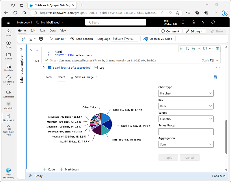
The built-in charting functionality in notebooks is useful when you want to quickly summarize the data visually. When you want to have more control over how the data is formatted, you should consider using a graphics package to create your own visualizations.

Using graphics packages in code

There are many graphics packages that you can use to create data visualizations in code. In particular, Python supports a large selection of packages; most of them built on the base Matplotlib library. The output from a graphics library can be rendered in a notebook, making it easy to combine code to ingest and manipulate data with inline data visualizations and markdown cells to provide commentary.

For example, you could use the following PySpark code to aggregate data from the hypothetical products data explored previously in this module, and use Matplotlib to create a chart from the aggregated data.

Python
from matplotlib import pyplot as plt

# Get the data as a Pandas dataframe
data = spark.sql("SELECT Category, COUNT(ProductID) AS ProductCount \
                  FROM products \
                  GROUP BY Category \
                  ORDER BY Category").toPandas()

# Clear the plot area
plt.clf()

# Create a Figure
fig = plt.figure(figsize=(12,8))

# Create a bar plot of product counts by category
plt.bar(x=data['Category'], height=data['ProductCount'], color='orange')

# Customize the chart
plt.title('Product Counts by Category')
plt.xlabel('Category')
plt.ylabel('Products')
plt.grid(color='#95a5a6', linestyle='--', linewidth=2, axis='y', alpha=0.7)
plt.xticks(rotation=70)

# Show the plot area
plt.show()

The Matplotlib library requires data to be in a Pandas dataframe rather than a Spark dataframe, so the toPandas method is used to convert it. The code then creates a figure with a specified size and plots a bar chart with some custom property configuration before showing the resulting plot.

The chart produced by the code would look similar to the following image:

Screenshot of a bar chart showing product counts by category.

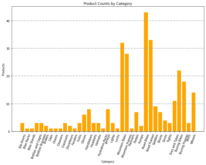
You can use the Matplotlib library to create many kinds of chart; or if preferred, you can use other libraries such as Seaborn to create highly customized charts.


Next unit: Exercise – Analyze data with Apache Spark